Program e-paper on the STM32L053-Discovery Board with the BSP Library using STM32CubeIDE

The purpose of this post is to demonstrate how to include the BSP library in a project and program the e-paper on an STM32L053-Discovery board. This method of including the BSP library is a modified version of the method described in the reference below.

References:

Versions Used:

  • STM32CubeIDE version 1.13.0
  • STM32Cube MCU Package for STM32L0 series version 1.12.0

In order to write to the e-paper included with the STM32L053-Discovery board, we need to connect the e-paper and microcontroller with an SPI for transmitting commands and data and a few GPIO lines for control. The needed connections are shown in the illustration below from application note AN4500 published by STMicroelectronics.

Figure 1 from AN4500 – How to display size-optimized pictures on a 4-grey level E-Paper from STM32 embedded memory (STMicroelectronics)

But we are lucky because all of this plus much more is taken care of by the BSP library distributed by STMicro.

Steps

  • Get BSP Library
  • Create Project with STM32CubeIDE
  • Configure Project
  • Add BSP Library to Project
  • Fix and Compile
  • Create Bitmap
  • Add Code to Upload Image to e-paper

Get BSP Library

The BSP library is included in STM32Cube MCU Package for STM32L0 series.

Download it from STMicro:

https://www.st.com/en/embedded-software/stm32cubel0.html

Un-zip the file. The BSP library for the STM32L053-Discovery board is in this folder:

..\en.stm32cubel0_v1-12-0\STM32Cube_FW_L0_V1.12.0\Drivers\BSP\STM32L0538-Discovery

It contains the following files:

There are some other files needed, but they are also included with the library.

Create New Project with STM32CubeIDE

Start STM32CubeIDE.

Create a new project by selecting File -> New -> STM32 Project from the menu:

This will open the STM32 Project – Target Selection window:

Select the MCU/MPU Selector tab (this is the default).

Find your processor using the filters, by paging down in the MCUs/MPUs List panel, or by typing the part number in the Commercial Part Number text box (you only need to type a distinguishing portion of the part number, L053, in this case. See below).

Select the specific part number in the MCUs/MPUs List panel:

Select Next.

A further STM32 Project window will open:

Enter a project name and leave everything else as shown above.

Select Finish.

Once the project has been created, the project should open to the Device Configuration Tool:

If the Device Configuration Tool does not open, RMB on the E-Paper_BSP.ioc file in the Project Explorer and select Open from the context menu:

Configure Project

Steps

  • Enable serial wire debug (optional)
  • Enable SPI1

Enable Serial Wire Debug

Under Categories, select System Core -> SYS:

In the SYS Mode and Configuration panel, select Debug Serial Wire.

Leave everything else as default.

In the Pinout view panel, pins PA13 and PA14 will now be green and assigned for serial debug.

Enable SPI1

While still in the Device Configuration Tool, under Categories, select Connectivity -> SPI1:

Under SPI1 Mode and Configuration, change Mode to anything but disable:

Note that pins PA5 and PA7 have now been assigned to the SPI1 interface (other modes may initiate more pins).

Do not make any other changes to the SPI1 configuration. The BSP initialization function, BSP_EPD_Init(), will configure SPI1 for communication with the e-paper.

The reason we enabled SPI1 is:

  • to ensure that stm32l0xx_hal_spi.h and stm32l0xx_hal_spi.c are included in folder Drivers -> STM32L0xx_HAL_Driver. These are needed by the BSP library, but are not included in the Drivers folder unless one of the SPI communication ports is enabled.
  • so that HAL_SPI_MODULE_ENABLED will be defined in stm32l0xx_hal_conf.h and file stm32l0xx_hal_spi.h will be included in the correct place in that file.

Snippets from stm32l0xx_hal_conf.h with SPI1 enabled:

Of course, this is a ridiculous way to do it, but otherwise you will need to fight STM32CubeIDE to do it manually.

No other configuration of SPI1 is needed since this will be done within BSP. Note that you could just as well enable SPI2 because that will also achieve the same.

BSP initialization will also configure GPIO pins for e-paper communication and control.

Save the project (ctrl-s). This will save the project and also auto-generate code.

Add BSP Library to Project

Using Windows File Explorer, find the Drivers folder in the package downloaded above:

Using another instance of Windows File Explorer, find the STM32CubeIDE workspace and open the Drivers folder inside the project folder:

Copy the BSP folder from the downloaded package and paste it in the project Drivers folder:

Open up the BSP folder:

Delete the un-needed folders:

From within STM32CubeIDE, RMB on project name and select Refresh from the context menu:

The new folders should now be visible in the Project Explorer:

RMB on project name and select Properties from the context menu. This will open the project properties window:

Select C/C++ General -> Paths and Symbols from the tree:

Select the Includes tab and then select Add to add a new directory. An Add directory path window will open:

From the Add directory path window, select Add to all configurations and then select Workspace

This will open a Folder selection window showing all of the projects in the workspace (only one, in this case):

Expand the tree to reveal the project folder structure:

Select the BSP folder from the tree and then select OK to select the folder and return to the Folder selection window:

The Directory text box will now be populated with the path to the selected folder.

Select OK to return the Properties window:

In the same way, add the BSP/STM32L0538-Discovery path:

Select Apply and Close. The following dialog will open (unless you already selected the Remember my decision option previously):

Select Rebuild Index to rebuild the index and return to the Device Configuration Tool window:

Save the project (ctrl-s).

Fix and Compile

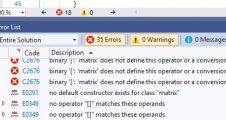
As configured, the project will not compile without error.

The problem is that there are multiple definitions of the fonts used in the BSP library (used to write text to the e-paper).

The easiest way to get around this issue is to comment out some include directives for font .c files in the stm32l0538_discovery_epd.h file. Like this:

Now the project will compile.

Create Bitmap

I created a bitmap suitable for the e-paper using GIMP.

Find an image that has a resolution the same or higher than the e-paper (72 x 172 pixels). Any format that GIMP can open will do. I just saved a screenshot as a .png file.

Open the file in GIMP:

(optional) Save the image in GIMP’s native image format (.xcf). To do this, select File -> Save (or ctrl-s):

Select Save to save the file.

Rotate the image by selecting Image -> Transform -> Rotate 90° clockwise:

The image after rotation:

Scale the image to match the e-paper resolution.

From the menu, select Image -> Scale Image – this will open the Scale Image window:

Change the Image Size units to px for pixels (was the default for me). The aspect ratio of the e-paper (172 px/72 px = 2.3889 ) and the image (677 px/412 px = 1.6432) do not match. Unless you don’t mind distorting the image, then some part of the image will be lost.

With the aspect ratio locked (the chain-link between the Width and Height should appear as shown above), try changing the width to 72 pixels. Press the Tab key or select the Height text box with the mouse to update the calculated Height pixel count:

The calculated Height pixel count is now less than 172 pixels. No good. We need 72 x 172.

Try changing the height to 172:

Okay, that works. We can just crop the image to 72 x 172. That’s next. For now, select Scale to scale the image and return to the main window:

Zoom in by holding ctrl and rotating the mouse wheel (pan by pressing the mouse wheel):

Select the crop tool (indicated by red rectangle below) or press shift-s:

With the crop tool selected, create a rough crop selection by clicking and dragging the mouse. The crop does not have to be accurate at this point:

Be sure that the position and size units are pixels (px), and then change the crop tool parameters to position (0, 0) and size (72, 172) as shown below:

The area of the image that will be cropped is shown as grayed:

To center the crop (if you wish to do so), increase the x-value of Position:

Double-click inside the rectangle to complete the crop:

The image resolution is now 72 pixels by 172 pixels. To save a copy in .xbm-format, select File -> Export from the menu:

You can change the name of the file by entering a new name in the Name text box (as was done above).

Expand Select File Type (By Extension) and scroll down to find the .xbm format:

Select the X BitMap image (xbm,icon,bitmap) format and then select Export. An options window will open:

Leave all options as default and select Export. The file should now be saved.

You can open the .xbm file with GIMP:

Obviously not a great choice of image, but good enough to demonstrate the method. And all that effort to carefully scale and crop the image without distortion!

This is what the file looks like in Notepad:

Add Code to Upload Image to e-paper

We need to add the project the contents of the .xbm file created above and other code to initialize the e-paper and upload the image.

In STM32CubeIDE, open the project’s main.c file. Scroll down to the user-code, private variable section:

Copy and paste the contents of the .xbm file between the BEGIN and END comments:

I renamed the image variable. You can delete the width and height definitions, if you wish, as they will not be used.

Open the main.h file and scroll down to the user-includes section:

Add #include “stm32l0538_discovery_epd.h” between the BEGIN and END comments, as shown above. This will add declarations for the functions needed to initialize the e-paper and to upload the image.

In the main.c file, scroll down to the user-code, section 2 in the main function:

Add BSP_EPD_INIT(); between the BEGIN and END comments, as shown above. This function will initialize the e-paper.

Now add this code:

BSP_EPD_Clear(EPD_COLOR_WHITE);
BSP_EPD_DrawImage(1, 1, 72, 172, image);
BSP_EPD_RefreshDisplay();

between the user-code while BEGIN and the while statement:

Now build the project.

Once the build is compete, run the project. The first time you run the project, a launch configuration window will open:

Keep the default settings and select OK.

Once the program has downloaded to the board, the screen should flash (that’s the BSP_EPD_Clear() function), and the hideous image should load:

But I prefer this image:

Simple Hit-Testing with wxWidgets

References:

  1. Original code: https://forums.wxwidgets.org/viewtopic.php?t=41893
  2. Hit-testing: https://www.xarg.org/book/computer-graphics/2d-hittest/
  3. Hit-testing in C#: https://learn.microsoft.com/en-us/dotnet/desktop/wpf/graphics-multimedia/hit-testing-in-the-visual-layer?view=netframeworkdesktop-4.8
  4. wxWidgets general reference book (free): https://www.wxwidgets.org/docs/book/
  5. Avoiding flicker: https://wiki.wxwidgets.org/Flicker-Free_Drawing
  6. R-tree: https://www.bartoszsypytkowski.com/r-tree/

As far as I can tell, wxWidgets does not provide general-purpose hit-testing on the client area of a window in the way that C# does [3].

This is the simplest implementation of hit-testing that I could devise. It is closely modeled on the code reference [1], but with most of the features stripped out to highlight the core features of hit-testing.

All that it does is perform a hit-test on a few lines drawn on a wxPanel. At each mouse move, a hit test is performed using the cursor location. If there is a hit on one or more of the lines, then it is or they are redrawn in red. Any line that was previously hit but is no longer is redrawn in blue.

This is a very crude version of hit-testing, where a hit is defined as the cursor position being inside the bounding box of a line. Typically, this is only the first step of a hit-test algorithm and is used to quickly find a subset of objects for more refined hit-testing. Some details of the next steps are explored in reference [2].

It’s fast because the bounding box is aligned with the coordinate system, so hit testing only requires checking if the cursor x-position is between the x-max and x-min of the bounding box and that the cursor y-position is between the y-max and y-min of the bounding box.

The three images below show what is looks like. The cursor is not visible, so you will just have to take my word for what is going on. The case with two lines hit is where the cursor is position in the overlap of the bounding boxes.

No hits:

Hit on one line:

Hit on two lines:

The lines are created and drawn during the application initialization (cApp::OnInit) and are fixed. The lines are created in cAppFrame::buildGeometry, and drawn in cAppFrame::draw.

Information on each line is stored in a structure (LineSegment) that contains the start and end points of the line and a boolean (m_Hit) that records if the line has been hit or not. As each line is created, it is added to a vector of lines (LineVector). This vector is used within a class (LineList) that provides the following functions:

  • AddLine adds a line to the vector
  • IsHit checks if the line was hit
  • SetHit sets the line as hit
  • SetNotHit sets the line as not hit
  • size returns the vector length
  • GetBndBox returns a wxRect that in the line’s bounding box
  • sp returns the starting point of the line
  • ep returns the ending point of the line

When the lines are drawn on the client area, the hit/not hit boolean is used to set the line color. Initially, no lines are hit so they are all drawn in blue.

Hit-testing is performed in response to a mouse movement event. Hit-testing involves stepping through the LineVector and checking if the mouse position is within the bounding rectangle of each line. If it is, m_Hit is set to true. If it isn’t, m_Hit is set to false. Actually, m_Hit is only set if the new condition is different from the last hit-testing. This was done to avoid redrawing at every mouse move.

If there are a large number of objects to be hit-tested, a more efficient data-structure than a vector may be needed. Something like an R-tree or similar, for example [6].

That’s about it.

Other Comments/Issues

  • To avoid flickering, the wxEraseEvent is handled with a handler that does nothing. I cannot find the reference where I found this idea, but it is discussed in references [4] and [5].
  • If you resize the window and make it larger, the wxMemoryDC bitmap is not resized, so the edge of the background drawn in the CAppFrame constructor will be visible.

Code Listing

The code consists of two files: a header file (.h) and a code file (.cpp).

Header file (cMain.h):

#pragma once

#include <wx/wx.h>
#include <wx/dcbuffer.h>


struct LineSegment
{
    LineSegment(const wxPoint& pt1, const wxPoint& pt2)
        : x1(pt1.x), y1(pt1.y), x2(pt2.x), y2(pt2.y) {}
    wxInt32 x1, y1, x2, y2;
    bool m_Hit = false;
};

typedef wxVector<LineSegment> LineVector;

class LineList
{
public:
    LineList() { }
    void AddLine(const wxPoint& pt1, const wxPoint& pt2) { m_lineVec.push_back(LineSegment(pt1, pt2)); }
    bool IsHit(int i) const { return m_lineVec[i].m_Hit; }
    void SetHit(int i) { m_lineVec[i].m_Hit = true; }
    void SetNotHit(int i) { m_lineVec[i].m_Hit = false; }
    const wxInt32 size() { return m_lineVec.size(); }
    wxRect GetBndBox(int i) { return wxRect(wxPoint(m_lineVec[i].x1, m_lineVec[i].y1), wxPoint(m_lineVec[i].x2, m_lineVec[i].y2)); }
    wxPoint sp(int i) { return wxPoint(m_lineVec[i].x1, m_lineVec[i].y1); }
    wxPoint ep(int i) { return wxPoint(m_lineVec[i].x2, m_lineVec[i].y2); }
private:
    LineVector m_lineVec;
};


class cApp : public wxApp
{
public:
        virtual bool OnInit() override;
};

class cAppFrame : public wxFrame
{
public:
    cAppFrame(const wxString& title);
    void buildGeometry();
    void draw();
private:
    void OnPaint(wxPaintEvent& event);
    void OnErase(wxEraseEvent& event) {};
    void OnMotion(wxMouseEvent& event);

    wxPanel* m_canvas;
    wxBitmap m_canvasBitmap;

    int m_canvasWidth, m_canvasHeight;

    LineList m_LineList;
};

Code file (cMain.cpp):

#include "cMain.h"


bool cApp::OnInit()
{
    cAppFrame* mainFrame = new cAppFrame(wxT("Line"));
    mainFrame->buildGeometry();
    mainFrame->draw();
    mainFrame->Show(true);
    return true;
}

void cAppFrame::buildGeometry()
{
    wxPoint sp = wxPoint(50, 60);
    wxPoint ep = wxPoint(150, 160);
    m_LineList.AddLine(sp, ep);

    sp = wxPoint(250, 80);
    ep = wxPoint(200, 10);
    m_LineList.AddLine(sp, ep);
    
    sp = wxPoint(40, 200);
    ep = wxPoint(70, 140);
    m_LineList.AddLine(sp, ep);
}

void cAppFrame::draw()
{
    wxMemoryDC dc(m_canvasBitmap);

    wxPen red = wxPen(*wxRED_PEN);
    wxPen blue = wxPen(*wxBLUE_PEN);
    const wxInt32 count = m_LineList.size();

    for (int i = 0; i < count; i++)
    {
        if (m_LineList.IsHit(i))
        {
            dc.SetPen(red);
        }
        else
        {
            dc.SetPen(blue);
        }
        dc.DrawLine(m_LineList.sp(i), m_LineList.ep(i));
    }
    m_canvas->Refresh();
}

void cAppFrame::OnPaint(wxPaintEvent& event)
{
    wxPaintDC(m_canvas).DrawBitmap(m_canvasBitmap, 0, 0);
}

void cAppFrame::OnMotion(wxMouseEvent& event)
{
    wxPoint mousePos = wxPoint(event.GetX(),event.GetY());
    wxRect boundingBox;

    const wxInt32 count = m_LineList.size();

    for (int i = 0; i < count; i++)
    {
        bool forceDraw = false;
        boundingBox = m_LineList.GetBndBox(i);
        if (boundingBox.Contains(mousePos))
        {
            if (!m_LineList.IsHit(i))
            {
                forceDraw = true;
                m_LineList.SetHit(i);
            }
        }
        else
        {
            if (m_LineList.IsHit(i))
            {
                forceDraw = true;
                m_LineList.SetNotHit(i);
            }
        }
        if (forceDraw) { this->draw(); }
    }
}

cAppFrame::cAppFrame(const wxString& title)
    :wxFrame(NULL, wxID_ANY, title, wxDefaultPosition, wxSize(600, 600))
{
    m_canvas = new wxPanel(this);
    this->Layout();
    this->SetBackgroundStyle(wxBG_STYLE_PAINT);

    m_canvasWidth = m_canvas->GetSize().GetWidth();
    m_canvasHeight = m_canvas->GetSize().GetHeight();

    m_canvasBitmap = wxBitmap(m_canvasWidth, m_canvasHeight, 24);
    wxMemoryDC dc(m_canvasBitmap);
    dc.SetPen(*wxWHITE_PEN);
    dc.SetBrush(*wxWHITE_BRUSH);
    dc.DrawRectangle(0, 0, m_canvasWidth, m_canvasHeight);

    m_canvas->Bind(wxEVT_PAINT, &cAppFrame::OnPaint, this);
    m_canvas->Bind(wxEVT_ERASE_BACKGROUND, &cAppFrame::OnErase, this);
    m_canvas->Bind(wxEVT_MOTION, &cAppFrame::OnMotion, this);
}

wxIMPLEMENT_APP(cApp);

Create minimal wxWidgets program from empty VS 2022 project

This procedure creates a minimal wxWidgets static-library app that does nothing useful, but provides a framework for building more complex apps. Here is what it looks like, in all its glory:

Versions Used:

  • Microsoft Visual Studio Community 2022, Version 17.4.1
  • wxWidgets 3.2.2.1

Main Reference:

Other References:

This procedure follows the explanation given in the YouTube video linked above, but with a few differences:

  • Uses an empty C++ project instead of a Windows desktop application.
  • Uses 64 bit library instead of 32 bit.
  • The app does not have a button, list-box, etc.

Download and install wxWidgets following the procedure from YouTube video linked above. Be sure to create the environment variable as shown in the video.

Steps:

  • Create empty C++ project
  • Add code for minimal app
  • Configure project to use wxWidgets library
  • Create project template

1. Create Empty C++ Project

From the menu-bar in VS, select Files -> New -> Project – this will open the Create a new project dialog:

Select Empty Project then select Next.

Enter a Project Name and select Create to generate the project.

2. Add Code for Minimal App

Once the project has generated, the Solution Explorer should look like this (with Project1 being replaced by the project name entered above):

RMB on the project name in the Solution Explorer to open a context menu:

From the context menu, select Add -> New Item – the Add New Item dialog should open:

Select Header File (.h) and then enter a name. In this case, the file name used was cMain.h

Enter the following code into the header file:

#pragma once
#include <wx/wx.h>

class MyProjectApp : public wxApp
{
public:
        virtual bool OnInit() override;
};

The IntelliSense will not be happy, and there will be red squiggly lines under wxApp, etc. Something like this:

This will be fixed once we add a path to the wxWindows library.

Add another file using Add -> New Item, only this time create a source code file by choosing file type C++ File (.cpp). Name the file using the same file name as the header file, but change the extension to .cpp.

Enter the following into the source code file:

#include "cMain.h"

bool MyProjectApp::OnInit()
{
    wxFrame* mainFrame = new wxFrame(nullptr, wxID_ANY, L"MyProject");
    mainFrame->Show(true);
    return true;
}
wxIMPLEMENT_APP(MyProjectApp);

3. Configure Project to Use wxWidgets Library

RMB on the project name in the Solution Explorer to open the context menu:

From the context menu, select Properties to open the Property Page dialog:

Along the top of the dialog, there is a drop-down to select which configurations any property changes should apply. Select All Configurations from the Configuration drop-down.

Select C/C++ -> General in the Configuration Properties tree (panel on the left side of dialog).

For the Select Additional Include Directories property, enter $(WXWIN)\include; $(WXWIN)\include\msvc

Note: $(WXWIN) is an environmental variable created during the wxWidgets tutorial in the YouTube video linked above.

Select C/C++ -> Precompiled Headers in the Configuration Properties tree:

For the Precompiled Header property, choose Not Using Precompiled Headers from the drop-down.

Select Linker in the Configuration Properties tree:

For the Additional Library Directories property, enter $(WXWIN)\lib\vc_x64_lib

Note: This is the 64 bit static library, rather than the 32 bit static library used in the video tutorial.

Select Linker -> System in the Configuration Properties tree:

For the SubSystem property, select Windows (/SUBSYSTEM:WINDOWS) from the pull-down (if needed, it may already be set to this).

Select OK.

The project should build and run without error.

The app should look like this:

Close the app and save the project (if you haven’t already).

4. Create Project Template

From the menu bar, select Project -> Export Template – the Export Template Wizard should open:

Select Next.

Enter a Template name. Select Finish to create the template.

The template should now be available when creating new projects, although you will need to select All languages from the Create a new project dialog to find it. If, for example, the template was named wxWidgets, then it should appear in the Create a new project dialog like this:

Select wxWidgets and then Next and proceed as usual to start a new project.

WPF/C# Ribbon with commands, hotkeys, and unsaved document flag.

This post demonstrates the rudiments of an app with ribbon control.

References:

This is what the finished app will look like:

The full code for this app is listed at the end of this post.

Create a Project:

Create C# WPF project. In this case, the project name is “Ribbon_Demo”. Note that whenever this project name is referred to, substitute the name of your project.

Build the Ribbon:

To use the ribbon control, we need to add the windows ribbon reference.

From Solution Explorer, select right mouse button (RMB) on Ribbon_DemoReferences.

Select Add Reference from the context menu – the Reference Manager dialog will open:

Scroll down and select System.Windows.Controls.Ribbon.

Select OK.

Add the following code to MainWindow.xaml:

<Ribbon>
    <RibbonTab Header="Home" KeyTip="H">
        <RibbonGroup Header="File">
        </RibbonGroup>
        <RibbonGroup Header="Edit">
        </RibbonGroup>
    </RibbonTab>
    <RibbonTab Header="Insert" KeyTip="I">
    </RibbonTab>
</Ribbon>

For reference, this is what MainWindow.xaml looked like in my project after I added the code. The rest of the code is auto-generated (everything except what is in the box above):

<Window x:Class="Ribbon_Demo.MainWindow"
        xmlns="http://schemas.microsoft.com/winfx/2006/xaml/presentation"
        xmlns:x="http://schemas.microsoft.com/winfx/2006/xaml"
        xmlns:d="http://schemas.microsoft.com/expression/blend/2008"
        xmlns:mc="http://schemas.openxmlformats.org/markup-compatibility/2006"
        xmlns:local="clr-namespace:Ribbon_Demo"
        mc:Ignorable="d"
        Title="MainWindow" Height="450" Width="800">
        <Ribbon>
            <RibbonTab Header="Home" KeyTip="H">
                <RibbonGroup Header="File">
                </RibbonGroup>
                <RibbonGroup Header="Edit">
                </RibbonGroup>
            </RibbonTab>
            <RibbonTab Header="Insert" KeyTip="I">
            </RibbonTab>
        </Ribbon>
 </Window>

Note that I deleted the Grid that is automatically generated when I create a new WPF project.

The above code will create two ribbon tabs, Home and Insert; with two ribbon groups, File and Edit, within the first tab.

Compile and run. The app should look like this:

You can switch between tabs by selecting each with the left mouse button (LMB).

Pressing Alt with the app running will bring up the key tips (indicated by arrows below). Selecting [H] or [I] on the keyboard switches between tabs.

These key tips were defined with KeyTip=”H” and KeyTip=”I” in the code above. Close the app.

Button with application command:

Add the following code to MainWindow.xaml inside the File ribbon group (refer to the full listing below to clarify where it should be added):

<RibbonButton Label="Close"
        Command="ApplicationCommands.Close"
        SmallImageSource="Resources/Close_16x.png"
        KeyTip="C"
        ToolTip="Close ( Ctrl+C )"/>

This will add a button with associated application command (“ApplicationCommands.Close”), an icon (“Resources/Close_16x.png”), a key tip (“C”), and a tool tip (“Close ( Ctrl+C )”).

Before we can compile and run the app, we need to add the “Close_16x.png” file as a resource.

Start by creating a new folder to contain the file:

From the Solution Explorer, RMB on Ribbon_Demo. From the context menu, select AddNew Folder:

Name the folder whatever you like, but I named it Resources:

Copy the “Close_16x.png” image from the VS2017 Image Library  to the Resources folder created above. I found the close image in the image library in folder Visual Studio 2019\Templates\VS2017 Image Library\VS2017\Close.

Now we need to add this file as a resource:

Within the Solution Explorer, RMB on Resources and from the context menu, select AddExisting Item:

The Add Existing Item dialog will open:

Navigate to the Resources folder.

From the pull-down, select Image Files and select the “Close_16x.png” file.

Select Add.

The code should compile and run, but it still doesn’t do anything interesting:

The Close ribbon button is grayed (and therefore disabled). Close the app.

Add Predefined Command with Action:

Now we add a command binding to the application command for Close along with two event handlers.

There are three types of commands available:

TypeDescription
Predefined commands with actionsome controls have commands with command bindings and action already implemented
Predefined commands without actioncommand is defined, but you need to do three things to make it work: 1. add a command binding, 2. define a function (handler) that determines if the command is disabled, and 3. define a handler that implements the action taken when the command is executed.
Custom commandsyou do all the work

Only the second two types of command will be used here, with the predefined command without action illustrated first.

Add the following to MainWindow.xaml just above* the Ribbon definition:

<Window.CommandBindings>
    <CommandBinding
        Command="ApplicationCommands.Close"
        CanExecute="CloseCommand_CanExecute"
        Executed="CloseCommand_Executed" />
</Window.CommandBindings>

*Gives the commands global scope.

This does three things:

  • 1. Binds the application command Close.
  • 2. Binds a CanExecute handler that is used to determine if the command is disabled.
  • 3. Binds an Executed handler that implements the command.

Now define the two functions (handlers). The name of the functions must match the attributes for CanExecute and Executed defined above.

Add the following code to the MainWindow class in MainWindow.xaml.cs:

private void CloseCommand_CanExecute(object sender, CanExecuteRoutedEventArgs e)
{
    e.CanExecute = true;
}
private void CloseCommand_Executed(object sender, ExecutedRoutedEventArgs e)
{
     MessageBox.Show("Close Command.",
         "Command", MessageBoxButton.YesNo, MessageBoxImage.Exclamation);
}

For reference, this is what MainWindow.xaml.cs looked like in my project after I added the code:

using System;
using System.Collections.Generic;
using System.Linq;
using System.Text;
using System.Threading.Tasks;
using System.Windows;
using System.Windows.Controls;
using System.Windows.Data;
using System.Windows.Documents;
using System.Windows.Input;
using System.Windows.Media;
using System.Windows.Media.Imaging;
using System.Windows.Navigation;
using System.Windows.Shapes;

namespace Ribbon_Demo
{
    /// <summary>
    /// Interaction logic for MainWindow.xaml
    /// </summary>
    public partial class MainWindow : Window
    {
        public MainWindow()
        {
            InitializeComponent();
        }
        private void CloseCommand_CanExecute(object sender, CanExecuteRoutedEventArgs e)
        {
            e.CanExecute = true;
        }
        private void CloseCommand_Executed(object sender, ExecutedRoutedEventArgs e)
        {
            MessageBox.Show("Close Command.",
                "Command", MessageBoxButton.YesNo, MessageBoxImage.Exclamation);
        }
    }
}

Note that most of the using directives are unnecessary, but are autogenerated when the project is created.

The added code does the following:

  • 1. CloseCommand_CanExecute  simply sets the CanExecute property to true. This means the command is always available.
  • 2. CloseCommand_Executed opens a message box to demonstrate that the command was invoked.

Now when the code is compiled and run, the Close button is enabled:

And a message box opens when the Close button is selected:

Select Yes and then close the app.

Add a HotKey:

Add the code shown below to the MainWindow class:

static MainWindow()
{
        // add hotkey to application command
        ApplicationCommands.Close.InputGestures.Add(
                new KeyGesture(Key.C, ModifierKeys.Control));
}

This defines a static MainWindow constructor containing an input gesture to the application command Close.

Now pressing Cntl+C will also activate the Close command.

Add a custom command:

This will be demonstrated using an Edit button with custom command.

First, add an Edit button to the ribbon by adding the following code to the Edit RibbonGroup within MainWindow.xaml,

<RibbonButton Label="Edit"
    Command="{x:Static local:MainWindow.CommandEdit}"
    SmallImageSource="Resources/Edit_16x.png"
    KeyTip="E"
    ToolTip="Edit ( Ctrl+E )"
    />

Note that this also includes an edit icon file that will have to be copied into the Resources folder and added to the project as a resource (as was done above for the close icon).

Now add the following command binding to Window.CommandBindings within MainWindow.xaml,

<CommandBinding
    Command="{x:Static local:MainWindow.CommandEdit}"
    CanExecute="EditCommand_CanExecute"
    Executed="ExecuteEdit"/>

Similar but not identical to the application command Close illustrated above, this does three things:

  • Binds to an as yet undefined custom command.
  • Binds a CanExecute handler that is used to determine if the command is disabled.
  • Binds an Executed handler that implements the command.

Next, define the custom command and handlers.

In MainWindow.xaml.cs we need to add four things:

1. A custom command object to the MainWindow class:

public readonly static RoutedUICommand CommandEdit;

2. Instantiate the custom command within the MainWindow static constructor:

CommandEdit = new RoutedUICommand("_Edit",
    "Edit Command", typeof(MainWindow));

3. Add a input gesture to the command within the MainWindow static constructor:

CommandEdit.InputGestures.Add(
    new KeyGesture(Key.E, ModifierKeys.Control));

4. Define the handlers in the MainWindow class:

private void ExecuteEdit(Object sender, ExecutedRoutedEventArgs e)
{
}
private void EditCommand_CanExecute(Object sender, CanExecuteRoutedEventArgs e)
{
    e.CanExecute = true;
}

The code should compile and run, but the Edit button will not do anything because ExecuteEdit is empty:

Add a Flag:

To make the Edit button a little more exciting, we will add an is-edited flag that is set to true when the Edit button is pressed, and set to false when the Close button is pressed. All this does is disable the Edit button once it has been pressed, and then enable it once the Close button is pressed.

First, add the flag to the MainWindow constructor:

private bool m_IsEdited = false;

It is initialized to false until the Edit button is pressed.

Modify the Edit handlers as shown below,

private void ExecuteEdit(Object sender, ExecutedRoutedEventArgs e)
{
    m_IsEdited = true;
}
private void EditCommand_CanExecute(Object sender, CanExecuteRoutedEventArgs e)
{
    e.CanExecute = (m_IsEdited == false);
}

Now ExecuteEdit sets the is-edited flag to true when the Edit button is pressed, and EditCommand_CanExecute disables the Edit button whenever the is-edited flag is true.

Modify the CloseCommand_Executed handler as follows,

private void CloseCommand_Executed(object sender, ExecutedRoutedEventArgs e)
{
    if (m_IsEdited)
    {
        if (MessageBox.Show("Unsaved changes. Close and loose changes?",
            "Unsaved Changes", MessageBoxButton.YesNo, MessageBoxImage.Exclamation)
                == MessageBoxResult.No) return;
    }
    m_IsEdited = false;
}

Now the Close button does nothing unless the is-edited flag is true (okay, it sets the flag to false, but it already was, so nothing changed).

If the is-edited flag is true, then pressing Close will display a message box. Pressing the Yes button on the message box closes it and sets the is-edited flag to false, but pressing the No button closes the message box but short-circuits the if statement with return, returning from the handler without setting the flag to false

To see this in action, compile and run the code.

Press the Edit button to disable it:

Now press the Close button. The message box will open:

Press Yes to enable the Edit button and No to keep it disabled.

That’s it.


Full code:

XAML code:

<Window x:Class="Ribbon_Demo.MainWindow"
        xmlns="http://schemas.microsoft.com/winfx/2006/xaml/presentation"
        xmlns:x="http://schemas.microsoft.com/winfx/2006/xaml"
        xmlns:d="http://schemas.microsoft.com/expression/blend/2008"
        xmlns:mc="http://schemas.openxmlformats.org/markup-compatibility/2006"
        xmlns:local="clr-namespace:Ribbon_Demo"
        mc:Ignorable="d"
        Title="MainWindow" Height="450" Width="800">
    <Window.CommandBindings>
        <CommandBinding
            Command="ApplicationCommands.Close"
            CanExecute="CloseCommand_CanExecute"
            Executed="CloseCommand_Executed" />
            <CommandBinding
                Command="{x:Static local:MainWindow.CommandEdit}"
                CanExecute="EditCommand_CanExecute"
                Executed="ExecuteEdit"/>
    </Window.CommandBindings>
    <Ribbon>
        <RibbonTab Header="Home" KeyTip="H">
            <RibbonGroup Header="File">
                <RibbonButton Label="Close"
                    Command="ApplicationCommands.Close"
                    SmallImageSource="Resources/Close_16x.png"
                    KeyTip="C"
                    ToolTip="Close ( Ctrl+C )"/>
            </RibbonGroup>
            <RibbonGroup Header="Edit">
                <RibbonButton Label="Edit"
                    Command="{x:Static local:MainWindow.CommandEdit}"
                    SmallImageSource="Resources/Edit_16x.png"
                    KeyTip="E"
                    ToolTip="Edit ( Ctrl+E )"
                    />
            </RibbonGroup>
        </RibbonTab>
        <RibbonTab Header="Insert" KeyTip="I">
        </RibbonTab>
    </Ribbon>
 </Window>

C# code:

using System;
using System.Collections.Generic;
using System.Linq;
using System.Text;
using System.Threading.Tasks;
using System.Windows;
using System.Windows.Controls;
using System.Windows.Data;
using System.Windows.Documents;
using System.Windows.Input;
using System.Windows.Media;
using System.Windows.Media.Imaging;
using System.Windows.Navigation;
using System.Windows.Shapes;

namespace Ribbon_Demo
{
    /// <summary>
    /// Interaction logic for MainWindow.xaml
    /// </summary>
    public partial class MainWindow : Window
    {
        public MainWindow()
        {
            InitializeComponent();
        }

        // Custom command objects.
        public readonly static RoutedUICommand CommandEdit;

        private bool m_IsEdited = false;

        static MainWindow()
        {
            // add hotkey to application command
            ApplicationCommands.Close.InputGestures.Add(
                new KeyGesture(Key.C, ModifierKeys.Control));
            // instantiate custom command and hotkey
            CommandEdit = new RoutedUICommand("_Edit",
                "Edit Command", typeof(MainWindow));
            CommandEdit.InputGestures.Add(
                new KeyGesture(Key.E, ModifierKeys.Control));

        }
        private void CloseCommand_CanExecute(object sender, CanExecuteRoutedEventArgs e)
        {
            e.CanExecute = true;
        }
        private void CloseCommand_Executed(object sender, ExecutedRoutedEventArgs e)
        {
            if (m_IsEdited)
            {
                if (MessageBox.Show("Unsaved changes. Close and loose changes?",
                    "Unsaved Changes", MessageBoxButton.YesNo, MessageBoxImage.Exclamation)
                        == MessageBoxResult.No) return;
            }
            m_IsEdited = false;
        }
        private void ExecuteEdit(Object sender, ExecutedRoutedEventArgs e)
        {
            m_IsEdited = true;
        }
        private void EditCommand_CanExecute(Object sender, CanExecuteRoutedEventArgs e)
        {
            e.CanExecute = (m_IsEdited == false);
        }
    }
}

Add Resources (Images, etc.) to VS 2019 Project

Create Resource Folder

Open the Solution Explorer tab in the Solution Explorer panel:

RMB on the solution name (Ribbon_Demo, in this example). From the context menu, select AddNew Folder:

Name the folder, in this example Resources. The folder should now appear in the solution tree:

Move Resources to Folder

In Windows Explorer, copy the resource(s), “Close_16x.png” image in this example, to the Resources folder created above.

Add File as Resource

Open the Solution Explorer tab in the Solution Explorer panel:

RMB on resource folder name (Resources in this example), and from the context menu, select AddExisting Item:

The Add Existing Item dialog will open:

Navigate to the folder containing the resource (Resources, in this example).

From the pull-down, select the file type to be added (Image Files, in this example) and select the file.

Select Add to close the dialog and add the resource to the solution.

Rotate tetrahedron around coordinate axis

Very simple, but inefficient and unscalable rotation of tetrahedron about y-axis with no hidden line removal.

References:

Tetrahedron is constructed with four points (vertices) and six lines (edges).

The algorithm:

  • Each point is rotated about the y-axis using a transform matrix.
  • Six lines are plotted on the xy-plane using rotated points.

The projection is accomplished by simply throwing away the z-coordinate of each point (parallel projection looking along the +z-axis).

Import needed modules:

Define the extent of the plot, turn on grid, plot coordinate axes with labels:

Out:

Define four points for the vertices (homogeneous coordinates):

Generate a matrix where each row has two points to define the tetrahedron edges:

Out:

Turn on interactive mode and get current instance of axes:

Current instance of axes is needed to remove lines from plot, preserving the grid, axes, and axis labels. Alternatively, matplotlib.pyplot.clf() will clear everything, but the grid, etc. will need to be re-initiated/plotted.

Now loop through rotation angles, plotting tetrahedron at each angle.

What is going on:

  • Loop through angles:
    • Delete existing lines in plot using current instance of axes
    • Create a rotation matrix using the current angle (after converting the angle to radians)
    • Loop through tetrahedron edges:
      • Rotate two points defining an edge
      • Plot xy-coordinates of these rotated points as a line
    • Pause for .02 seconds so that us poor humans can see the rotation

Output at angle 0°:

Full listing:

import matplotlib.pyplot as plt
import numpy as np
from math import sin, cos, pi

# plot axis, grid, coordinate axes and labels in figure
plt.axis([-3,3,3,-3])
plt.axis('on')
plt.grid(True)
plt.arrow(0,0,2,0,head_length=.5,head_width=.2,color='k')
plt.arrow(0,0,0,2,head_length=.5,head_width=.2,color='k')
plt.text(2.5,-.5,'x')
plt.text(-.5,2.5,'y')

# generate vertices of tetrahedron
a, b, c, d = (-1,-1,0,1), (2,-2,0,1), (-0.5,1,-4,1), (0.5,3,0,1)

# generate matrix of lines for the tetrahedron edges
E = np.array([[a,b]
            ,[b,c]
            ,[c,d]
            ,[d,a]
            ,[d,b]
            ,[c,a]])

# turn on interactive mode
plt.ion()
# get current instance of axes
ax = plt.gca()

# loop to rotate tetrahedron
for angle in range(0,361,5): # loop though angles
    # delete any existing lines in plot
    for x in range(len(ax.lines)):
        ax.lines.remove(ax.lines[0])
        plt.draw()
    # create rotation matrix
    θ = angle/180*pi
    rot=np.array(((cos(θ),0,sin(θ),0),
					 (0,1,0,0),
					 (-sin(θ),0,cos(θ),0),
					 (0,0,0,1)))
    for x in E: # loop through edges
        # rotate points defining tetrahedron edges
        s=np.array([ np.matmul(rot,x[0,:]), np.matmul(rot,x[1,:]) ])
        # plot pairs of points as line
        ll=plt.plot(s[:,0],s[:,1],color='b')
    plt.pause(.02) # slow loop

Delete line from matplotlib.pyplot

Two of many ways to do this:

  • delete all lines
  • delete one line using the line instance

Delete all lines

Import needed modules (numpy is only used to generate data):

Generate dummy data and plot:

Creates this plot:

Get current instance of current axes:

Loop through all lines and delete them:

You may think that this could be written as:

but this will not work as the iterable is being changed by the loop itself.

A full listing with pauses to allow visualizing the lines being deleted:

import matplotlib.pyplot as plt
import numpy as np

# plot lines
plt.plot(np.arange(0,10,1), 'g--o')
plt.plot(np.arange(0,20,2), 'r--o')
plt.plot(np.arange(0,30,3), 'b--o')

# get current instance of axes
ax = plt.gca()

for x in range(len(ax.lines)):
    plt.pause(1)
    print(ax.lines[0],'\n')
    # remove line
    ax.lines.remove(ax.lines[0])
    # redraw figure
    plt.draw()

The addition of plt.draw() is required to redraw the plot after each line is removed.

Delete one line using the line instance

import matplotlib.pyplot as plt
import numpy as np

line1, = plt.plot(np.arange(0,10,1), 'b--s')
line2, = plt.plot(np.arange(0,20,2), 'ro')
line3, = plt.plot(np.arange(0,30,3), 'bo')

ax = plt.gca()

ax.lines.remove(line1)

In this case, each plot returns the Line2D instance of the line that can be used to delete the line.

Implementation of discrete radon transform (parallel beam geometry)

The radon transformation was taken directly from https://gist.github.com/fubel/ad01878c5a08a57be9b8b80605ad1247, but with tweaks to allow variable steps in transform.

The back-projection is a crude reverse of the forward transformation. This is an unfiltered back projection.

Code:

import numpy as np
import matplotlib.pyplot as plt
from skimage.transform import rotate

def discrete_radon_transform(image, steps):
    R = np.zeros((image.shape[0],steps), dtype='float')
    for s in range(steps):
        rotation = rotate(image, -s*180/steps).astype('float')
        R[:,s] = sum(rotation)
    return R

def discrete_inv_radon_transform(R):
    steps = R.shape[1]
    image = np.zeros((R.shape[0],R.shape[0]), dtype='float')
    update = np.zeros((R.shape[0],R.shape[0]), dtype='float')
    for s in range(steps):
        update[:,:] = R[:,s]
        rotation = rotate(update, s*180/steps).astype('float')
        image = image + rotation
    return image

# generate simple image
image =np.zeros((400,400))
image[40:50,100:110]=255

# standard test image
#from skimage.data import shepp_logan_phantom
#image = shepp_logan_phantom()

steps = 500

aspect = steps/image.shape[0] # to keep sinogram plot square

radon = discrete_radon_transform(image, steps)
inv_radon = discrete_inv_radon_transform(radon)

# Plot the original image, sinogram, and backprojected sinogram
plt.figure(figsize=(20,20))

plt.subplot(1, 3, 1), plt.imshow(image, cmap='gray')
plt.xticks([]), plt.yticks([])

plt.subplot(1, 3, 3), plt.imshow(inv_radon, cmap='gray')
plt.xticks([]), plt.yticks([])

plt.subplot(1, 3, 2), plt.imshow(radon, cmap='gray',aspect = aspect)
plt.xticks([]), plt.yticks([])

Output (original image, sinogram, back-projection):

Now using a standard test image (uncomment lines 27 and 28):

Multiple Regression: Using PyTorch to Generate Regression Coefficients

This example generates parameters for a second order polynomial that fits synthetic data.

The main source for this example comes from:

https://donaldpinckney.com/books/pytorch/book/ch2-linreg/2018-03-21-multi-variable.html

which has a good explanation of the underlying concepts, and a deeper explanation of the algorithm itself.

Other sources for details on plotting and data generation are:

https://www.kaggle.com/kanncaa1/pytorch-tutorial-for-deep-learning-lovers

https://www.guru99.com/pytorch-tutorial.html

The code

Import modules:

Print version numbers:

Output:

Generate Data

Now generate the synthetic data. In this example, the underlying model is a second-order polynomial, with added random noise.

Define the underlying noiseless model:

There is nothing special about the constants chosen, so pick your favorites.

Now some parameters that define the number of data points, the maximum x value, and the amplitude of the noise:

Use these parameters to generate a NumPy array of random x-values and use the x-values values to generate corresponding NumPy array of y-values:

Note that the noise is adjusted to center at zero.

Now plot the generated data:

Output:

In this plot–and subsequent plots–the clean y-data is plotted as a blue line, and the noisy y-data is plotted as green circles.

I am using Spyder so had to change the default setting in Spyder so that the plots would appear in separate windows. This step is not necessary and a bad idea if you are plotting a lot of figures. Anyway, see this link for instructions on how to do this:

https://www.scivision.dev/spyder-with-ipython-make-matplotlib-plots-appear-in-own-window/

You will need to re-start the kernel after making this change.

Now we need to reconfigure the generated data for use in PyTorch.

Because we generated the data, we already know the underlying model, a second-order polynomial. For this regression, we will also assume a second-order polynomial (cheating, yes). The independent variables for this polynomial are x and x2, so we need an array with two rows: one with the x-values generated above and one with them squared.

These values do not change during training.

Now convert this and the y-values from a NumPy array to a PyTorch tensor:

Define the Model

A second-order polynomial has three coefficients, two for the  x and x2 variables (A), plus one that defines the intersection with the y-axis (b). Since, obviously, we do not know these values yet, we initiate them with random values:

Output:

Define a function that generates y-values using the current estimated values of A and b and the x and x2 values generated above.

Define the loss function and optimizer.

In this example, the loss function is constructed, but PyTorch has a good number built-in, including a mean squared error function that is the same as this function (nn.MSELoss with reduction = ‘sum’). See https://pytorch.org/docs/stable/nn.html#loss-functions for more.

And now plot predicted y-values using the randomly initialized values of A and b:

This function, plot_state, is defined in the full code listing at the end of this post.

Output:

The predicted y-values are plotted with magenta circles. Even with randomly initiated coefficients, the polynomial shape is apparent.

Before we can train the model, we need to define some parameters:

where loss_list is an array to capture the losses for display later, num_iterations is self-explanatory, and num_plots defines how many times to plot current predicted y-values during training.

Now training:

Output after first iteration:

Output after 500 iterations:

After the 500th iteration, the estimated coefficients of the polynomial are 98.1, 4.3, and 4.8, while the coefficients used to generate the synthetic data were 100, 2, and 5. Although the coefficients of the y-intercept and x2 are reasonably close, the coefficient of x is way off. Perhaps this is not surprising given that the y-intercept is much larger than the x-coefficient, and that a function of x2 will dominate a function of x, if their coefficients are of the same order of magnitude. In addition, the amplitude of the noise is quite large and reducing its amplitude improves the fit (it had better). Or maybe there is something wrong with the code.

Now plot the loss over iterations:

Output:

The loss drops very quickly in the first 50 or so iterations, but is still declining at over 400 iterations. Reducing the synthetic data y-intersect speeds up the convergence.

Full code listing:

"""
from: https://donaldpinckney.com/books/pytorch/book/ch2-linreg/2018-03-21-multi-variable.html
plotting: https://www.kaggle.com/kanncaa1/pytorch-tutorial-for-deep-learning-lovers
data generation and plotting: https://www.guru99.com/pytorch-tutorial.html
"""

# import modules
import matplotlib
import matplotlib.pyplot as plt
import torch
import torch.optim as optim
import numpy as np

# print module versions
import sys # only used to print python version
print('Python: ',sys.version)
print('torch: ',torch.__version__)
print('matplotlib: ',matplotlib.__version__)
print('numpy: ',np.__version__)

####################################################################
# generate synthetic data
####################################################################

# define noiseless underlying model
def y_clean(x_input):
    return 10 + 2*x_input + 5*np.power(x_input,2)

# generate synthetic data 
num_x = 50 # number of x points (also batch size)
x_max = 8 # maximum value (minimum = 0)
noise = 50 # random noise amplitude
x = x_max*np.random.rand(num_x) # generate random x values
x = np.sort(x) # to make plotting easier
y = y_clean(x) + noise*np.random.rand(num_x)-(noise/2)

# plot noisy data
plt.figure()
plt.plot(x,y_clean(x),'b')
plt.scatter(x,y,c='g')
plt.xlabel("x values")
plt.ylabel("output")
plt.title("Clean and Noisy Input")
plt.show()

# generate array with x and x^2 rows
x_dataset_np = np.stack((np.power(x,1),np.power(x,2)),axis=0)

# convert numpy array to pytorch tensor
x_dataset = torch.from_numpy(x_dataset_np).float()
y_dataset = torch.from_numpy(y).float()

####################################################################
# define plotting function that display current predicted values
####################################################################

def plot_state(x_data,y_data,xx,iteration):
    plt.figure()

    y_predict = model(x_data).data.numpy()
    
    plt.scatter(xx,y_predict[0,:],c='m')
    plt.scatter(xx,y_data[:],c='g')
    plt.plot(xx,y_clean(xx),'b-')
    plt.title(f"Iteration  {iteration}")
    plt.xlabel("x values")
    plt.ylabel("output")
    plt.show()
    
####################################################################
# define PyTorch model
####################################################################

n = 2 # define degree of polynomial
torch.manual_seed(1) # ensures a consistent sequence of pseudo-random numbers
# assign random values to initial polynomial parameters (A,b) 
A = torch.randn((1, n), requires_grad=True)
b = torch.randn(1, requires_grad=True)
print(A,b)

# define model
def model(x_input):
    return A.mm(x_input) + b

# define batch loss function
def loss(y_predicted, y_target):
    return ((y_predicted - y_target)**2).sum()

# define the optimizer 
optimizer = optim.Adam([A, b], lr=2.5)

# plot predicted output using randomly initialized parameters, A and b
plot_state(x_dataset,y_dataset,x,0)

####################################################################
# train
####################################################################
loss_list = []
num_iterations =500
num_plots = 4 # number of plots per run
nn = int(num_iterations / num_plots)

for t in range(num_iterations):
    
    # zero out gradients
    optimizer.zero_grad() 
    
    # calculate output using current polynomial parameters (A,b)
    y_predicted = model(x_dataset) 
    
    # calculate sum of squared error
    current_loss = loss(y_predicted, y_dataset) 
    
    # calculate the loss gradient
    current_loss.backward()
    
    # update polynomial parameters (A,b)
    optimizer.step()
    
    # store loss
    loss_list.append(current_loss.data)
    
    if (t % nn == 0)or(t == (num_iterations-1)):
        print(f"t = {t+1}, loss = {current_loss}, A = {A.detach().numpy()}, b = {b.item()}")
        plot_state(x_dataset,y_dataset,x,t+1)

# plot loss versus iterations
plt.figure()
plt.plot(range(num_iterations),loss_list)
plt.xlabel("Number of Iterations")
plt.ylabel("Loss")
plt.title("Loss vs. Iterations")
plt.yscale("log")
plt.grid(True,which="both" )
plt.show()

Classification in OpenCV Using Pre-built Caffe Model

Based upon:

  1. https://becominghuman.ai/face-detection-with-opencv-and-deep-learning-90b84735f421

With additional input from:

2. https://www.pyimagesearch.com/2017/08/21/deep-learning-with-opencv/

3. https://nbviewer.jupyter.org/github/BVLC/caffe/blob/master/examples/00-classification.ipynb

A) Download Caffe Models

Need the following three files:

  1. .prototxt file containing model definition
  2. .caffemodel file containing layer weights
  3. a synset file containing category labels

and an image file. Just steal one from the internet like everyone else does (or free from www.pexels.com).

Before going any further, create a project folder to contain Caffe model files and Python script. Also save the image file to the project folder.

Download .prototex and .caffemodel files

Link to files:

https://github.com/BVLC/caffe/tree/master/models/bvlc_googlenet

This will open a page looking something like this:

LMB on caffemodel_url to download .caffemodel file. Copy file from Downloads folder to project folder.

LMB on “deploy.prototxt”. This will open a page listing the contents of this file. RMB on [Raw] and select “Save link as . . .” to download the .prototex file. Save the file in the project folder. I renamed it “bvlc_googlenet_deploy.prototxt” to identify it with the model.

Download synset file

The following link will download the tar file containing synset file:

http://dl.caffe.berkeleyvision.org/caffe_ilsvrc12.tar.gz

Move file from Downloads folder to project folder. Then extract it to a separate folder within project folder (tar file contains more than just synset file).

B) Python Code

Create new python script file in project folder. Copy the code below into that file (or paste into IPython, or similar console).

Import modules and print versions:

import numpy as np
import cv2 as cv
import sys # only used to print python version
print('Python: ',sys.version)
print('numPy: ',np.version)
print('OpenCV: ',cv.version)

Output:

Python: 3.7.3 (default, Apr 24 2019, 15:29:51) [MSC v.1915 64 bit (AMD64)]
numPy: 1.16.4
OpenCV: 4.1.1

Define model filenames:

PROTOTXT = 'bvlc_googlenet_deploy.prototxt'
MODEL = 'bvlc_googlenet.caffemodel'

Define confidence level:

CONFIDENCE = .4

This defines the minimum level that constitutes a successful classification.

Load model:

net = cv.dnn.readNetFromCaffe(PROTOTXT, MODEL)

Load class label file and extract labels to array:

rows = open('_labels/synset_words.txt').read().strip().split("\n")
classes = [r[r.find(" ") + 1:].split(",")[0] for r in rows]

Load image file:

img = cv.imread('example.jpg')

Calculate image mean:

imgM = cv.mean(img)
print('image mean ',imgM)

Output (mean-R, mean-G, mean-B, ???) :

image mean (135.6633213531514, 153.53549636533464, 168.6211724333983, 0.0)

Generate 4D blob from image:

blob = cv.dnn.blobFromImage(img , 1.0, (224, 224), imgM)

where the parameters for this command are:

  • scale factor = 1.0
  • size of output image = (224, 224)
  • mean of image to be subtracted

Run the blob though the model:

net.setInput(blob)
detections = net.forward()

Extract predictions:

idxs = np.argsort(detections[0])[::-1][:5]

Loop over the top 5 predictions and print the label and probability:

for (i, idx) in enumerate(idxs):
   # print predicted label and probability to console
   print("({}) {}, p = {:.5}".format(i + 1,
      classes[idx], detections[0][idx]))
   # write label and prediction for most likely category on image
   if i == 0:
      text = "{}, p={:.2f}%".format(classes[idx],
         detections[0][idx] * 100)
      cv.putText(img, text, (5, 25), cv.FONT_HERSHEY_SIMPLEX,
         0.7, (0, 0, 255), 2)

Output:

(1) Labrador retriever, p = 0.51849
(2) Chesapeake Bay retriever, p = 0.35624
(3) German short-haired pointer, p = 0.048037
(4) curly-coated retriever, p = 0.032651
(5) vizsla, p = 0.023717

Display image:

cv.imshow('img', img)

Wait for any key to be pressed, and then close window

cv.waitKey()
cv.destroyAllWindows()

Output:

Code list:

import numpy as np
import cv2 as cv
import sys # only used to print python version
print('Python: ',sys.version)
print('numPy: ',np.__version__)
print('OpenCV: ',cv.__version__)

# define model filenames
PROTOTXT = 'bvlc_googlenet_deploy.prototxt'
MODEL = 'bvlc_googlenet.caffemodel'

# detection parameters
CONFIDENCE = .4

# load model from disk
net = cv.dnn.readNetFromCaffe(PROTOTXT, MODEL)

# Load class label file and extract labels to array
rows = open('_labels/synset_words.txt').read().strip().split("\n")
classes = [r[r.find(" ") + 1:].split(",")[0] for r in rows]

# load image file
img = cv.imread('example.jpg')

# calculate image mean
imgM = cv.mean(img)
print('image mean ',imgM)

# generate 4-D blob from image
# scale factor = 1.0
# size of output image = (224, 224)
# mean of image to be subtracted (mean-R, mean-G, mean-B)
blob = cv.dnn.blobFromImage(img , 1.0, (224, 224), imgM)

# run blob though model
net.setInput(blob)
detections = net.forward()

# Extract predictions
idxs = np.argsort(detections[0])[::-1][:5]

# Loop over the top 5 predictions and print the label and probability
for (i, idx) in enumerate(idxs):
   # print predicted label and probability to console
   print("({}) {}, p = {:.5}".format(i + 1,
      classes[idx], detections[0][idx]))
   # write label and prediction for most likely category on image
   if i == 0:
      text = "{}, p={:.2f}%".format(classes[idx],
         detections[0][idx] * 100)
      cv.putText(img, text, (5, 25), cv.FONT_HERSHEY_SIMPLEX,
         0.7, (0, 0, 255), 2)

# Display image
cv.imshow('img', img)

# wait for any key to be pressed, and then close window
cv.waitKey()
cv.destroyAllWindows()

Design a site like this with WordPress.com
Get started